Velocity Verlet: Symplecticity and Energy Behavior
Velocity Verlet is one of the standard integrators in molecular dynamics. Its update equations are simple, but the explanation for why it works so well often involves less familiar terms: Liouville operators, symplecticity, and shadow Hamiltonians. What do these ideas actually mean, and how do they explain the energy we observe in a simulation?
In this post, we will build these ideas from Hamilton’s equations. We will first derive the algorithm by splitting the motion into simpler pieces, then examine its accuracy and the geometry it preserves. Finally, we will work through a harmonic oscillator, where we can calculate the energy error and the stability limit exactly. This will give us a practical basis for choosing a time step.
Prerequisite: Hamilton’s equations and basic calculus. Operators and the geometric meaning of symplecticity will be introduced along the way.
From Hamilton’s Equations to the Liouville Operator
Consider a particle with position $q$, momentum $p$, and constant mass $m>0$. We assume a smooth, time-independent, separable Hamiltonian
\[H(q,p)=T(p)+V(q)=\frac{p^2}{2m}+V(q).\]Here, $T$ is the kinetic energy and $V$ is the potential energy. Hamilton’s equations give
\[\dot q=\frac{\partial H}{\partial p}=\frac{p}{m}, \qquad \dot p=-\frac{\partial H}{\partial q}=-V'(q)=F(q).\]We will use one spatial coordinate to keep the derivations readable, and explain the extension to many particles when discussing symplecticity. Throughout, $h=\Delta t$ is a fixed time step, and $(q_n,p_n)$ is the numerical state at $t_n=nh$.
An operator is a rule for differentiating an observable
Suppose we want to follow a quantity $A(q,p)$ along a trajectory. This quantity, called an observable, could be position, momentum, or energy. If $A$ has no explicit time dependence, the chain rule gives
\[\begin{aligned} \frac{dA}{dt} &=\frac{\partial A}{\partial q}\dot q +\frac{\partial A}{\partial p}\dot p\\ &=\frac{p}{m}\frac{\partial A}{\partial q} -V'(q)\frac{\partial A}{\partial p}. \end{aligned}\]The same differentiation rule applies to every observable. Using the conventional Liouville operator notation, we write
\[i\mathcal L =\frac{p}{m}\frac{\partial}{\partial q} -V'(q)\frac{\partial}{\partial p}, \qquad \frac{dA}{dt}=i\mathcal L A.\]Here, $\mathcal L$ is the Liouville operator, and $i\mathcal L$ is the evolution generator. The factor $i$ is part of this conventional definition: the combination $i\mathcal L$ is a real differential operator, so it does not make classical positions or momenta complex.
Another common notation is the Poisson bracket, defined by
\[\{A,B\} =\frac{\partial A}{\partial q}\frac{\partial B}{\partial p} -\frac{\partial A}{\partial p}\frac{\partial B}{\partial q}.\]Thus, $i\mathcal L A=\lbrace A,H\rbrace$. This is simply the chain-rule result written in a compact form. As a quick check,
\[i\mathcal L q=\frac{p}{m}, \qquad i\mathcal L p=-V'(q),\]which recovers Hamilton’s equations.
Why does an exponential describe the motion?
The expression $i\mathcal L A$ is itself a function of $q$ and $p$. We can apply the same chain rule to this new function:
\[\begin{aligned} \frac{d^2A}{dt^2} &=\frac{d}{dt}\bigl(i\mathcal L A\bigr)\\ &=\frac pm\frac{\partial(i\mathcal L A)}{\partial q} +F(q)\frac{\partial(i\mathcal L A)}{\partial p}\\ &=(i\mathcal L)(i\mathcal L A)=(i\mathcal L)^2A. \end{aligned}\]Repeating this argument gives $d^kA/dt^k=(i\mathcal L)^kA$. The assumption of no explicit time dependence matters: otherwise, differentiating $i\mathcal L A$ would also introduce an explicit time derivative of the operator. Taylor expansion along the trajectory now gives
\[\begin{aligned} A(q(t+h),p(t+h)) &=\left[A+h(i\mathcal L)A+\frac{h^2}{2}(i\mathcal L)^2A+\cdots\right]_{(q(t),p(t))}\\ &=\left[e^{ih\mathcal L}A\right]_{(q(t),p(t))}. \end{aligned}\]The exponential is shorthand for the operator series
\[e^{ih\mathcal L} =I+h(i\mathcal L)+\frac{h^2}{2}(i\mathcal L)^2+\cdots,\]where $I$ leaves an observable unchanged. For a general smooth system, we use this series as a local expansion; the exact evolution operator itself is defined by following the exact trajectory.
For example, applying the operator twice to position gives
\[\begin{aligned} (i\mathcal L)q &=\frac pm\underbrace{\frac{\partial q}{\partial q}}_{1} +F(q)\underbrace{\frac{\partial q}{\partial p}}_{0} =\frac pm,\\ (i\mathcal L)^2q &=(i\mathcal L)\left(\frac pm\right)\\ &=\frac pm\underbrace{\frac{\partial(p/m)}{\partial q}}_{0} +F(q)\underbrace{\frac{\partial(p/m)}{\partial p}}_{1/m} =\frac{F(q)}m. \end{aligned}\]Substituting these derivatives into the series gives
\[q(t+h)=q(t)+h\frac{p(t)}{m}+\frac{h^2}{2m}F(q(t))+O(h^3).\]The operator exponential has reproduced the usual Taylor expansion of position. Here, $O(h^3)$ means that the omitted terms are bounded in magnitude by a constant times $h^3$ as $h\to0$, in the region under consideration.
Splitting the Motion into Drift and Kick
Writing the exact solution as $e^{ih\mathcal L}$ is useful, but it does not automatically tell us how to calculate it. The practical advantage appears when we split the generator into its kinetic and potential contributions:
\[i\mathcal L=i\mathcal L_T+i\mathcal L_V, \qquad i\mathcal L_T=\frac{p}{m}\frac{\partial}{\partial q}, \qquad i\mathcal L_V=F(q)\frac{\partial}{\partial p}.\]Each part describes a simpler Hamiltonian system that we can solve exactly.
Under $T(p)$ alone, Hamilton’s equations become
\[\dot q=\frac{\partial T}{\partial p}=\frac pm, \qquad \dot p=-\frac{\partial T}{\partial q}=0.\]The second equation gives $p(t+s)=p(t)$ throughout this substep. Therefore,
\[q(t+\tau)-q(t) =\int_0^\tau\frac{p(t+s)}m\,ds =\int_0^\tau\frac{p(t)}m\,ds =\tau\frac{p(t)}m.\]This is the drift map
\[D_\tau(q,p)=\left(q+\tau\frac{p}{m},p\right).\]Under $V(q)$ alone, the equations instead become
\[\dot q=\frac{\partial V}{\partial p}=0, \qquad \dot p=-\frac{\partial V}{\partial q}=F(q).\]Now $q(t+s)=q(t)$, so the force stays constant during the substep, even when $F$ is a nonlinear function of position. Integrating gives
\[p(t+\tau)-p(t) =\int_0^\tau F(q(t+s))\,ds =\tau F(q(t)).\]This is the kick map
\[K_\tau(q,p)=\left(q,p+\tau F(q)\right).\]Here, $D_\tau$ names the drift map on states; the Liouville operators continue to be denoted by $\mathcal L_T$ and $\mathcal L_V$. An observable is advanced by evaluating it at the new state, so the two observable propagators are
\[\begin{aligned} e^{i\tau\mathcal L_T}A(q,p)&=A\left(q+\tau\frac{p}{m},p\right),\\ e^{i\tau\mathcal L_V}A(q,p)&=A\left(q,p+\tau F(q)\right). \end{aligned}\]The full dynamics changes position and momentum simultaneously. Splitting replaces that coupled motion with a sequence of exact drifts and kicks.
Why does the order matter?
If we kick first and then drift, the drift uses the updated momentum. If we drift first and then kick, the kick uses the updated position. The two results are generally different.
In operator language, $i\mathcal L_T$ and $i\mathcal L_V$ do not commute: applying them in opposite orders can give different answers. An operator product acts on its argument from right to left. For example,
\[\begin{aligned} (i\mathcal L_T)(i\mathcal L_V)q &=(i\mathcal L_T)\left(F(q)\frac{\partial q}{\partial p}\right) =(i\mathcal L_T)0=0,\\ (i\mathcal L_V)(i\mathcal L_T)q &=(i\mathcal L_V)\left(\frac pm\right) =F(q)\frac{\partial(p/m)}{\partial p} =\frac{F(q)}m. \end{aligned}\]This prevents us from using the ordinary scalar identity $e^{a+b}=e^ae^b$. To see where it fails, abbreviate $X=i\mathcal L_T$ and $Y=i\mathcal L_V$. These are temporary names for the generators, not new physical quantities. Since we must retain the order of multiplication,
\[(X+Y)^2=(X+Y)(X+Y)=X^2+XY+YX+Y^2.\]Expanding the exact propagator therefore gives
\[e^{h(X+Y)} =I+h(X+Y)+\frac{h^2}{2}(X^2+XY+YX+Y^2)+O(h^3).\]But multiplying two separate exponentials gives
\[\begin{aligned} e^{hX}e^{hY} &=\left(I+hX+\frac{h^2}{2}X^2+O(h^3)\right) \left(I+hY+\frac{h^2}{2}Y^2+O(h^3)\right)\\ &=I+h(X+Y)+h^2\left(\frac{X^2}{2}+XY+\frac{Y^2}{2}\right)+O(h^3). \end{aligned}\]The $XY$ term comes from multiplying $hX$ in the first factor by $hY$ in the second. There is no $YX$ term because the factors are never reversed. Subtracting the exact series gives
\[\begin{aligned} e^{hX}e^{hY}-e^{h(X+Y)} &=h^2\left(XY-\frac12XY-\frac12YX\right)+O(h^3)\\ &=\frac{h^2}{2}(XY-YX)+O(h^3). \end{aligned}\]A single full drift and full kick therefore generally has an error of order $h^2$ per step.
The symmetric splitting
To give both orderings a chance to appear, try a symmetric composition with as-yet unknown coefficients $b$ and $c$:
\[e^{bhY}e^{chX}e^{bhY} =I+h(cX+2bY)+O(h^2).\]Matching the linear term $h(X+Y)$ requires $c=1$ and $2b=1$. Thus, the first and last kicks must each have duration $h/2$, while the drift has duration $h$:
\[S_h=e^{i\frac h2\mathcal L_V}e^{ih\mathcal L_T}e^{i\frac h2\mathcal L_V} =e^{\frac h2Y}e^{hX}e^{\frac h2Y}.\]This is called Strang splitting. Matching the linear term only establishes consistency; we still need to check the quadratic terms. First multiply the left and middle factors:
\[\begin{aligned} e^{\frac h2Y}e^{hX} &=\left(I+\frac h2Y+\frac{h^2}{8}Y^2+O(h^3)\right) \left(I+hX+\frac{h^2}{2}X^2+O(h^3)\right)\\ &=I+h\left(X+\frac Y2\right) +h^2\left(\frac{X^2}{2}+\frac{YX}{2}+\frac{Y^2}{8}\right)+O(h^3). \end{aligned}\]Now multiply this result by the final half-kick factor. The quadratic terms come from three places: the quadratic terms already present, products of the two linear terms, and the quadratic term in the last factor:
\[\begin{aligned} S_h &=I+h\left(X+\frac Y2+\frac Y2\right)\\ &\quad+h^2\left[ \left(\frac{X^2}{2}+\frac{YX}{2}+\frac{Y^2}{8}\right) +\left(X+\frac Y2\right)\frac Y2+\frac{Y^2}{8} \right]+O(h^3)\\ &=I+h(X+Y)\\ &\quad+h^2\left[ \frac{X^2}{2}+\frac{YX}{2}+\frac{XY}{2} +\left(\frac18+\frac14+\frac18\right)Y^2 \right]+O(h^3)\\ &=I+h(X+Y)+\frac{h^2}{2}(X^2+XY+YX+Y^2)+O(h^3)\\ &=e^{ih\mathcal L}+O(h^3). \end{aligned}\]The two mixed terms now have the correct coefficients. Both subproblems are solved exactly, while their composition approximates the full motion through second order.
Recovering Velocity Verlet and Its Error Order
In terms of states, the symmetric step is
\[\Phi_h=K_{h/2}\circ D_h\circ K_{h/2},\]where the rightmost map acts first. Applying the three maps gives
\[\boxed{ \begin{aligned} p_{n+1/2}&=p_n+\frac h2F(q_n),\\ q_{n+1}&=q_n+\frac hmp_{n+1/2},\\ p_{n+1}&=p_{n+1/2}+\frac h2F(q_{n+1}). \end{aligned}}\]These are the Velocity Verlet equations. The label $p_{n+1/2}$ denotes the intermediate momentum used by the algorithm; it need not equal the exact physical momentum at $t_n+h/2$.
We can also eliminate the intermediate momentum explicitly. Substituting the first line of Velocity Verlet into the second gives
\[\begin{aligned} q_{n+1} &=q_n+\frac hm\left(p_n+\frac h2F(q_n)\right)\\ &=q_n+h\frac{p_n}m+\frac{h^2}{2m}F(q_n). \end{aligned}\]Substituting it into the third line gives
\[\begin{aligned} p_{n+1} &=\left(p_n+\frac h2F(q_n)\right)+\frac h2F(q_{n+1})\\ &=p_n+\frac h2\left[F(q_n)+F(q_{n+1})\right]. \end{aligned}\]Finally, dividing the momentum equation by the constant mass and setting $v=p/m$ gives the more familiar form
\[\begin{aligned} q_{n+1}&=q_n+hv_n+\frac{h^2}{2m}F(q_n),\\ v_{n+1}&=v_n+\frac{h}{2m}\left[F(q_n)+F(q_{n+1})\right]. \end{aligned}\]Once the initial force is known, each step requires only one new force evaluation: the force at $q_{n+1}$ can be reused at the beginning of the next step.
Local error versus global error
Our splitting calculation shows that, starting from the exact state, one numerical step differs from one exact step by $O(h^3)$. This is the local error.
Over a fixed simulation time, the number of steps grows like $1/h$. For smooth dynamics with bounded error amplification over that interval, accumulating the one-step errors gives the global error:
\[\text{global trajectory error}=O(h^{-1}h^3)=O(h^2).\]This makes Velocity Verlet a second-order method: halving $h$ typically reduces the trajectory error by about a factor of four once the step is sufficiently small.
The fixed-time qualification matters: this estimate does not guarantee that the numerical trajectory stays close to the exact trajectory indefinitely.
Reversing the step
A drift is undone by a drift of duration $-\tau$:
\[D_{-\tau}(D_\tau(q,p)) =D_{-\tau}\left(q+\tau\frac pm,p\right) =\left(q+\tau\frac pm-\tau\frac pm,p\right)=(q,p).\]Likewise, a kick leaves $q$ fixed, so the inverse kick uses the same force:
\[K_{-\tau}(K_\tau(q,p)) =\left(q,p+\tau F(q)-\tau F(q)\right)=(q,p).\]The inverse of a composition must undo the last operation first. Thus,
\[\Phi_h^{-1} =K_{h/2}^{-1}\circ D_h^{-1}\circ K_{h/2}^{-1} =K_{-h/2}\circ D_{-h}\circ K_{-h/2} =\Phi_{-h}.\]Thus, Velocity Verlet is symmetric in time: a step forward followed by the same algorithm with $-h$ returns to the original state in exact arithmetic. For our Hamiltonian, reversing momentum also reverses the motion. To verify this, define $R(q,p)=(q,-p)$ and calculate
\[\begin{aligned} R D_h R(q,p) &=R D_h(q,-p)=R\left(q-h\frac pm,-p\right)=D_{-h}(q,p),\\ R K_h R(q,p) &=R K_h(q,-p)=R(q,-p+hF(q))=K_{-h}(q,p). \end{aligned}\]Since $R^2=I$, inserting $R^2$ between the substeps then gives $R\Phi_hR=\Phi_{-h}$.
Time symmetry and second-order accuracy are useful properties. To understand the long-time energy behavior, however, we also need to examine what happens to phase space.
What Does Symplecticity Mean?
A state is a point $(q,p)$ in phase space. Imagine a small patch of nearby initial states and follow how it moves. The patch may stretch, tilt, or change shape. For one degree of freedom, a map is symplectic if it preserves the oriented area of every such patch.
How does a transformation change phase-space area?
Consider a general map
\[(q,p)\longrightarrow\bigl(Q(q,p),P(q,p)\bigr).\]Take a very small displacement $(dq,dp)$. To first order, the corresponding change in the new coordinates is
\[\begin{aligned} dQ&=\frac{\partial Q}{\partial q}\,dq +\frac{\partial Q}{\partial p}\,dp,\\ dP&=\frac{\partial P}{\partial q}\,dq +\frac{\partial P}{\partial p}\,dp. \end{aligned}\]We can collect these derivatives into the Jacobian matrix:
\[\begin{pmatrix}dQ\\dP\end{pmatrix} =\underbrace{\begin{pmatrix} \dfrac{\partial Q}{\partial q}&\dfrac{\partial Q}{\partial p}\\[4pt] \dfrac{\partial P}{\partial q}&\dfrac{\partial P}{\partial p} \end{pmatrix}}_{J} \begin{pmatrix}dq\\dp\end{pmatrix}.\]Now take a tiny rectangle with edges $(dq,0)$ and $(0,dp)$. The map turns these edges into
\[\left(\frac{\partial Q}{\partial q}dq,\frac{\partial P}{\partial q}dq\right), \qquad \left(\frac{\partial Q}{\partial p}dp,\frac{\partial P}{\partial p}dp\right).\]These span a parallelogram. The signed area spanned by two planar vectors $(a,b)$ and $(c,d)$ is $ad-bc$, so its new area is
\[\begin{aligned} dA_{\mathrm{new}} &=\left( \frac{\partial Q}{\partial q}\frac{\partial P}{\partial p} -\frac{\partial Q}{\partial p}\frac{\partial P}{\partial q} \right)dq\,dp\\ &=(\det J)\,dA. \end{aligned}\]Here, $dA=dq\,dp$ is the original area. Thus $\det J=1$ means that the map preserves both area and orientation. In one degree of freedom, this is the condition for symplecticity.
Why Hamiltonian motion preserves this area
Over a short time $\delta t$, Hamilton’s equations give the following Taylor expansion of the exact motion:
\[Q=q+\delta t\frac{\partial H}{\partial p}+O(\delta t^2), \qquad P=p-\delta t\frac{\partial H}{\partial q}+O(\delta t^2).\]Differentiating with respect to the initial $q$ and $p$ gives
\[J=\begin{pmatrix} 1+\delta t\dfrac{\partial^2H}{\partial q\,\partial p} &\delta t\dfrac{\partial^2H}{\partial p^2}\\[6pt] -\delta t\dfrac{\partial^2H}{\partial q^2} &1-\delta t\dfrac{\partial^2H}{\partial p\,\partial q} \end{pmatrix}+O(\delta t^2).\]In its determinant, the product of the off-diagonal entries is of order $\delta t^2$. Keeping the terms through first order gives
\[\begin{aligned} \det J &=1+\delta t\left( \frac{\partial^2H}{\partial q\,\partial p} -\frac{\partial^2H}{\partial p\,\partial q} \right)+O(\delta t^2)\\ &=1+O(\delta t^2). \end{aligned}\]The mixed derivatives cancel because $H$ is smooth. Consequently, the instantaneous rate of area change is
\[\frac{d(dA)}{dt} =\lim_{\delta t\to0}\frac{dA_{\mathrm{new}}-dA}{\delta t} =\lim_{\delta t\to0}\frac{\det J-1}{\delta t}\,dA =0.\]This holds at every point and every time, so the exact motion preserves area over a finite time interval as well. In one degree of freedom, Hamiltonian motion is therefore symplectic.
Why drift and kick preserve it exactly
For the drift map,
\[Q=q+\frac\tau m p, \qquad P=p.\]Its derivatives give
\[J_D=\begin{pmatrix}1&\tau/m\\0&1\end{pmatrix}, \qquad \det J_D=1\cdot1-\frac\tau m\cdot0=1.\]For the kick map,
\[Q=q, \qquad P=p+\tau F(q),\]so
\[J_K=\begin{pmatrix}1&0\\\tau F'(q)&1\end{pmatrix}, \qquad \det J_K=1\cdot1-0\cdot\tau F'(q)=1.\]Both substeps preserve area exactly for any $\tau$. The chain rule says that the Jacobian of a composition is the product of the substep Jacobians, evaluated at the corresponding intermediate states. Determinants multiply, so for Velocity Verlet’s kick–drift–kick step,
\[\det J_{\mathrm{VV}} =\det J_{K,\mathrm{second}}\, \det J_D\, \det J_{K,\mathrm{first}} =1.\]Velocity Verlet is symplectic because it is a composition of exact Hamiltonian subflows. Here the Jacobian calculation verifies this directly, with no small-step approximation.
Notice that a nonsymmetric kick–drift composition would also be symplectic, even though it is only first-order accurate. Symplecticity and accuracy order describe different properties.
What changes for many particles?
For many particles, we apply the same drift and kick rules to every position–momentum pair $(q_i,p_i)$. Here, $i$ labels a coordinate component; a particle moving in three dimensions has three such pairs.
\[\begin{aligned} \text{drift:}\qquad &q_i\longmapsto q_i+\tau\frac{p_i}{m_i}, &&p_i\longmapsto p_i,\\ \text{kick:}\qquad &q_i\longmapsto q_i, &&p_i\longmapsto p_i-\tau\frac{\partial V}{\partial q_i}. \end{aligned}\]The potential $V$ can depend on all the positions, so each particle’s force can depend on the other particles. During a kick, all positions are held fixed, so these forces remain constant and the momentum update is exact. During a drift, all momenta are held fixed, so the position update is exact.
These are again exact Hamiltonian subflows: the drift follows $T=\sum_i p_i^2/(2m_i)$, and the kick follows $V$. We use the general result that exact Hamiltonian flows are symplectic in any number of dimensions, and that composing symplectic maps preserves this property. Therefore, Velocity Verlet remains symplectic for interacting many-particle systems.
Why the Energy Can Oscillate
For the exact dynamics, energy conservation follows immediately from Hamilton’s equations:
\[\frac{dH}{dt} =H_q\dot q+H_p\dot p =H_qH_p-H_pH_q=0.\]Equivalently, $i\mathcal L H=\lbrace H,H\rbrace=0$. Every higher power also vanishes, since applying the operator to zero gives zero. Hence,
\[e^{ih\mathcal L}H =H+h(i\mathcal L)H+\frac{h^2}{2}(i\mathcal L)^2H+\cdots=H.\]Velocity Verlet uses a different propagator. A kick changes the kinetic energy while holding position fixed; a drift changes the potential energy while holding momentum fixed. Each substep conserves its own sub-Hamiltonian, but generally changes the total $H=T+V$. Applying the previously derived splitting error to the smooth observable $H$ gives
\[S_hH=e^{ih\mathcal L}H+O(h^3)=H+O(h^3).\]Since $(S_hH)(q_n,p_n)=H(q_{n+1},p_{n+1})$, this means
\[H(q_{n+1},p_{n+1})-H(q_n,p_n)=O(h^3).\]This explains the size of a one-step energy error. To understand what happens after many steps, we will work through a harmonic oscillator. The algebra will show exactly why Forward Euler accumulates energy error, while Velocity Verlet preserves a slightly modified energy.
Energy Behavior of a Harmonic Oscillator
Consider a particle attached to a spring, with Hamiltonian
\[H(q,p)=\frac{p^2}{2m}+\frac12m\omega^2q^2, \qquad F(q)=-m\omega^2q.\]Here, $\omega>0$ is the angular frequency. Hamilton’s equations are
\[\dot q=\frac pm, \qquad \dot p=-m\omega^2q.\]The exact motion continuously exchanges kinetic and potential energy while keeping their sum constant. For example, if we release the particle from $q_0=Q>0$ with $p_0=0$, then
\[q(t)=Q\cos(\omega t), \qquad p(t)=-m\omega Q\sin(\omega t).\]Substitution into $H$ gives
\[H(t)=\frac12m\omega^2Q^2 \left[\sin^2(\omega t)+\cos^2(\omega t)\right] =\frac12m\omega^2Q^2=H_0.\]We will now integrate the same equations numerically and write $H_n=H(q_n,p_n)$ for the physical energy after $n$ steps.
Forward Euler: energy grows at every step
Forward Euler uses the current derivatives to advance both variables:
\[q_{n+1}=q_n+h\frac{p_n}{m}, \qquad p_{n+1}=p_n-hm\omega^2q_n.\]Both right-hand sides use the old state $(q_n,p_n)$. This is the usual explicit Euler method; using an already updated variable in the other equation would give a different method.
Insert these updates into the energy and expand the squares:
\[\begin{aligned} H_{n+1} &=\frac{(p_n-hm\omega^2q_n)^2}{2m} +\frac{m\omega^2}{2}\left(q_n+h\frac{p_n}{m}\right)^2\\ &=\frac{p_n^2}{2m}-h\omega^2q_np_n +\frac{h^2m\omega^4q_n^2}{2}\\ &\quad+\frac{m\omega^2q_n^2}{2}+h\omega^2q_np_n +\frac{h^2\omega^2p_n^2}{2m}\\ &=H_n+h^2\omega^2 \left(\frac{p_n^2}{2m}+\frac{m\omega^2q_n^2}{2}\right). \end{aligned}\]The cross terms cancel, but the two terms proportional to $h^2$ are positive. Therefore,
\[\boxed{H_{n+1}=(1+h^2\omega^2)H_n.}\]Applying the same relation at every step gives
\[H_1=(1+h^2\omega^2)H_0, \qquad H_2=(1+h^2\omega^2)^2H_0, \qquad \boxed{H_n=(1+h^2\omega^2)^nH_0.}\]For any nonzero initial energy and any fixed $h>0$, the energy grows geometrically with the number of steps. The error accumulates because every step adds energy with the same sign. A smaller step slows this growth, but Forward Euler cannot sustain bounded oscillations indefinitely at any positive fixed step.
This also fits the geometric picture: its Jacobian is
\[J_{\mathrm E}=\begin{pmatrix}1&h/m\\-hm\omega^2&1\end{pmatrix}, \qquad \det J_{\mathrm E}=1+h^2\omega^2>1.\]Euler expands phase-space area at every step, and the numerical oscillator spirals outward.
Velocity Verlet: a nearby energy stays constant
For the same force, the kick–drift–kick equations become
\[\begin{aligned} p_{n+1/2}&=p_n-\frac h2m\omega^2q_n,\\ q_{n+1}&=q_n+\frac hm p_{n+1/2},\\ p_{n+1}&=p_{n+1/2}-\frac h2m\omega^2q_{n+1}. \end{aligned}\]Substituting the first equation into the second gives
\[q_{n+1}=\left(1-\frac{h^2\omega^2}{2}\right)q_n+\frac hm p_n.\]Combining the two kicks and then substituting this position gives
\[\begin{aligned} p_{n+1} &=p_n-\frac h2m\omega^2(q_n+q_{n+1})\\ &=\left(1-\frac{h^2\omega^2}{2}\right)p_n -hm\omega^2\left(1-\frac{h^2\omega^2}{4}\right)q_n. \end{aligned}\]For the next calculation, abbreviate the two repeated factors as
\[a=1-\frac{h^2\omega^2}{2}, \qquad \alpha=1-\frac{h^2\omega^2}{4}.\]Then the update is simply
\[q_{n+1}=aq_n+\frac hm p_n, \qquad p_{n+1}=ap_n-hm\omega^2\alpha q_n.\]The extra factor $\alpha$ suggests trying an energy with a slightly altered potential term:
\[\boxed{ I_h(q,p)=\frac{p^2}{2m}+\frac12m\omega^2\alpha q^2. }\]We can check this candidate directly. Multiply by $2m$ to remove the fractions, and substitute the update:
\[\begin{aligned} 2mI_h(q_{n+1},p_{n+1}) &=(ap_n-hm\omega^2\alpha q_n)^2 +m^2\omega^2\alpha\left(aq_n+\frac hm p_n\right)^2\\ &=a^2p_n^2-2ahm\omega^2\alpha q_np_n +h^2m^2\omega^4\alpha^2q_n^2\\ &\quad+m^2\omega^2\alpha a^2q_n^2 +2ahm\omega^2\alpha q_np_n +h^2\omega^2\alpha p_n^2\\ &=(a^2+h^2\omega^2\alpha) \left(p_n^2+m^2\omega^2\alpha q_n^2\right). \end{aligned}\]The cross terms cancel. The remaining factor is exactly one:
\[\begin{aligned} a^2+h^2\omega^2\alpha &=\left(1-\frac{h^2\omega^2}{2}\right)^2 +h^2\omega^2\left(1-\frac{h^2\omega^2}{4}\right)\\ &=1-h^2\omega^2+\frac{h^4\omega^4}{4} +h^2\omega^2-\frac{h^4\omega^4}{4}=1. \end{aligned}\]We have therefore proved
\[\boxed{I_h(q_{n+1},p_{n+1})=I_h(q_n,p_n).}\]Velocity Verlet exactly conserves this modified energy for the harmonic oscillator, in exact arithmetic with a fixed step. It resembles the physical energy, but the coefficient of $q^2$ differs by a term proportional to $h^2$.
Why the physical energy stays in a band
Subtracting the modified energy from the physical energy gives
\[\begin{aligned} H(q,p)-I_h(q,p) &=\frac12m\omega^2(1-\alpha)q^2\\ &=\frac{m\omega^4h^2}{8}q^2. \end{aligned}\]Since $I_h$ has the same value at every step, subtracting the initial energy from the energy at step $n$ leaves
\[\boxed{ H_n-H_0=\frac{m\omega^4h^2}{8}(q_n^2-q_0^2). }\]Compare this with Euler’s result. Here the error depends only on the difference between the current and initial squared positions. If the motion remains bounded, the energy error remains bounded too. As the particle moves back and forth, this correction oscillates instead of increasing at every step.
We can make the bound explicit for a particle released from rest, $q_0=Q$ and $p_0=0$. When $\alpha>0$, conservation of $I_h$ gives
\[\frac{p_n^2}{2m}+\frac12m\omega^2\alpha q_n^2 =\frac12m\omega^2\alpha Q^2.\]Both terms on the left are nonnegative, so $0\leq q_n^2\leq Q^2$. Using $H_0=\tfrac12m\omega^2Q^2$ in the energy-error formula yields
\[-\frac{(h\omega)^2}{4} \leq\frac{H_n-H_0}{H_0}\leq0, \qquad \boxed{\frac{\lvert H_n-H_0\rvert}{H_0}\leq\frac{(h\omega)^2}{4}.}\]This bound does not grow with the number of steps. Halving $h$ reduces the energy-error envelope by a factor of four. The fact that the energy stays below $H_0$ here comes from our choice to start at rest; other initial conditions can place $H_0$ elsewhere within the energy band.
For example, with $m=\omega=Q=1$ and $h=0.4$, we have $H_0=0.5$ and $I_h=0.48$. The physical energy stays between $0.48$ and $0.50$, while the modified energy stays at $0.48$. With $h=0.2$, the physical-energy interval narrows to $0.495\leq H_n\leq0.50$.
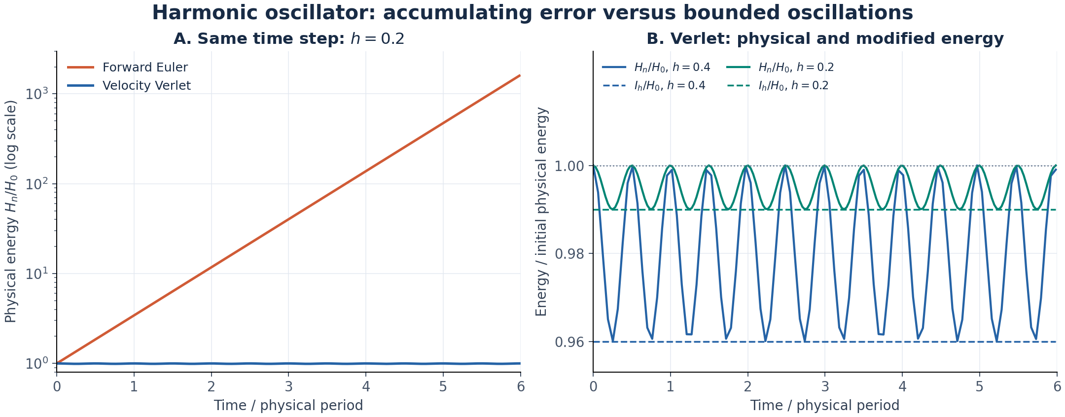
The oscillator gives us an unusually simple, exactly conserved modified energy. For more general smooth systems, the related idea is a nearby modified or shadow Hamiltonian that is nearly conserved over long times under suitable small, fixed-step conditions. We do not need its full construction here; the oscillator already shows how preserving a nearby energy can keep the physical-energy error bounded. The broader theory is discussed by Hairer, Lubich, and Wanner.
Choosing the Time Step
The conserved quantity also tells us why a symplectic method still needs a sufficiently small step.
Stay inside the stability limit
For $I_h$ to bound both position and momentum, its two squared terms must have positive coefficients. Thus we need
\[\alpha=1-\frac{h^2\omega^2}{4}>0 \quad\Longrightarrow\quad \boxed{0<h\omega<2.}\]In this range, a constant value of $I_h$ describes a closed ellipse in phase space, which confines the numerical trajectory. At $h\omega=2$, the coefficient of $q^2$ vanishes, so the conserved quantity no longer bounds position. Above that value, its level curves are hyperbolas rather than ellipses. For this oscillator, the strict inequality is the stability limit: generic trajectories can grow at the boundary and grow exponentially above it. Symplecticity by itself does not prevent that instability.
For a system with several approximately harmonic motions, the fastest angular frequency $\omega_{\max}$ gives the most restrictive condition:
\[h<\frac{2}{\omega_{\max}}.\]Stiff vibrations and light particles tend to set this fastest timescale. In a nonlinear system, the relevant timescales can change as the configuration changes, so this estimate is a starting point rather than a universal guarantee.
Choose accuracy well inside that limit
A stable trajectory can still have a large energy error. For our oscillator released from rest, the bound derived above gives:
| Step $h\omega$ | Steps per period $2\pi/(h\omega)$ | Relative energy-error envelope $(h\omega)^2/4$ |
|---|---|---|
| $0.1$ | $62.8$ | $0.25\%$ |
| $0.2$ | $31.4$ | $1\%$ |
| $0.5$ | $12.6$ | $6.25\%$ |
| $1.0$ | $6.3$ | $25\%$ |
For instance, keeping the energy deviation below one percent requires
\[\frac{(h\omega)^2}{4}\leq0.01 \quad\Longrightarrow\quad h\omega\leq0.2.\]Since one physical period is $2\pi/\omega$, this means roughly 32 or more steps per period. That is much more restrictive than merely requiring $h\omega<2$. The one-percent bound applies to this oscillator and initial condition, rather than to every molecular system.
Energy is also only one measure of accuracy. Verlet can keep the energy bounded while gradually getting ahead of or behind the exact oscillation. If the timing of the motion matters, check positions, frequencies, or time-dependent observables as well.
Check convergence in the actual simulation
Start with a fixed step that resolves the fastest motion, then repeat the calculation with $h/2$ over the same physical duration.
- Check energy in an NVE run: fixed particle number and volume, with no thermostat. For smooth dynamics in the second-order regime, integration-related energy fluctuations should shrink by roughly four when the step is halved.
- Compare the quantity you actually want to measure. Reduce the step further if that quantity changes appreciably. For chaotic systems, compare the relevant statistics with their sampling uncertainty rather than demanding that long trajectories stay identical.
- Investigate persistent energy drift. Inaccurate forces, abrupt potential cutoffs, poorly converged constraints, and roundoff can spoil the ideal behavior. A smaller step may not resolve all of these issues.
A thermostat or barostat exchanges energy with the system, so its physical $T+V$ need not stay constant in those simulations. This is why an NVE check is useful for assessing integration error. Keep the step fixed during these checks: changing it also changes the modified energy that the oscillator calculation conserves.
Enjoy Reading This Article?
Here are some more articles you might like to read next: